ShuffleNet > SqueezeNet > VGG
| Model | 핵심 Conv 형태 | 특징 | 장점 | 단점 |
| Xception | Depthwise separable conv | 깊이를 증가 | ||
| MobileNetV1 | Depthwise separable conv | 깊이대신 경량화 이슈 | ||
| ShuffleNet | Depthwise separable conv + Pointwise group conv + Channel shuffle | |||
| ResNeXt | Group conv | |||
| MobileNetV2 | Inverted Residual | Depthwise conv의 연산 비중을 늘림 + ReLU6 사용 | ||
| scaling up을 3가지 측면 (depth, channel width, resolution)을 조정 |
Depthwise Convolution
8x8x3의 matrix를 conv하기 위해서 3x3x3의 커널을 사용. 이때 각 채널별로 분리되어 3x3의 2차원 커널이 8x8 크기의 분리된 matrix에 붙어서 conv하고 다시 붙여지는 형태
쉽게 말해서 채널 방향의 Convolution은 하지 않고, 공간 방향의 convolution만 채널별로 진행

Depthwise Separable Convolution
Depthwise convolution + Pointwise Convolution을 결합한 것
처음 단계에서 진행된 Depthwise convolution 결과가, 각 채널을 1개로 압축할 수 있는 추가 convolution (즉 pointwise convolution)을 진행하여 경량화된 결과물이 나옴
이 때문에, 채널을 압축시키는 효과가 있어서 연산속도를 향상시킬 수 있다는 장점이 있음

Group Convolution
대표적인 Architecture인 ResNeXt의 차이만 보면 확연히 알 수 있음
기존 중간에 64개의 입력이 64개의 출력으로 나오는 반면,

Group convolution의 경우 입력 128개를 총 group = 32개 만큼, 즉 각 group당 4개의 입력 채널에 대해서만 convolution을 수행하여 총 4개의 output을 출력함
이렇게 하는 이유는? 서로 다른 특징 (흑백, 컬러)에 집중하여 학습이 가능함 (cardinality = 그룹수)
논문에서는 Group수를 증가시키는것이 한 그룹안에 channel수를 증가시키는 것보다 효율적이라고 언급하고 있음
Pointwise Group Convolution
1x1 pointwise convolution의 연산량을 감소시키기 위해서 제안

Channel Shuffle
Pointwise group conv을 사용할때 3x3 conv가 입력 채널 그룹에 대해서만 연산을 수행하고, 그에 관련된 정보만 출력하다보니, 채널 간의 정보 교환을 막기때문에 많은 정보를 이용할 수 없음
이 때문에 Channel shuffle이 제안됨
서로 다른 그룹에서 입력값을 받도록 함

아래의 그림은 shufflenet에서 구현하는 channel shuffle의 예

Squeeze and Excitation Block
아무런 Architecture에 SE Block을 붙여 넣을 수 있음
대표적 장점. 1. 유연성 (아무곳에 가능), 2. 추가계산량이 적음 (그러면서 성능 up)
직관적으로 이해하면 Architecture 중간에 또다른 tiny model을 넣은 느낌
SE Block을 넣음으로써 각 채널의 contribution을 파악하여 weight로 사용됨
약간의 파라미터 수의 증가량이 있지만, 성능 향상에 큰 도움을 줌
크게 두가지 과정 (Squeeze and Excitation)을 거침
Squeeze (짜내다): Global Information embedding
각 채널들의 중요한 정보만 추출해서 가져가겠다
Excitation: Adaptive recalibration
중요한 정보들을 압축 (squeeze) 했다면, 이번에는 재조정 (recalibration) 하는 단계
더 자세한 내용은 다음 링크 참조
SENet(Squeeze and excitation networks)알렉스넷이 나온 이후로 몇 년 동안은 ILSVRC에서 어떻게든 에러를 낮추기 위한 노력이 계속되었습니다. 그러나 레즈넷 이후로는 classification 분야에서는 네트워크 구조에 대한 관심이 많이 줄어들었습니다. 이번 포스트에서는 channel-wise feature response를 적절하게 조절해주는 "Squeeze-and-Excitation(SE)" 방법론을 제안한 SENet에 대하여 알아보도록 하겠습니다. CNN 네트워크를 잘 살펴보면, convolution filter 하나하나가 이미지 또는 피쳐맵의 "local"을 학습합니다.https://jayhey.github.io/deep%20learning/2018/07/18/SENet/

Fully-connected layer와 비선형 함수 (ReLU and sigmoid)를 이용하여 조절

def Squeeze_excitation_layer(self, input_x, out_dim, ratio, layer_name): with tf.name_scope(layer_name) : squeeze = Global_Average_Pooling(input_x) excitation = Fully_connected(squeeze, units=out_dim / ratio, layer_name=layer_name+'_fully_connected1') excitation = Relu(excitation) excitation = Fully_connected(excitation, units=out_dim, layer_name=layer_name+'_fully_connected2') excitation = Sigmoid(excitation) excitation = tf.reshape(excitation, [-1,1,1,out_dim]) scale = input_x * excitation return scale

RepVGG
Re-parameterization
여러 multiple module을 하나로 합쳐서 전체 네트워크가 plane-network (like VGG) 형태로 재탄생하게 됨
Linear Bottleneck (MobileNetv2에서 실시)
Depthwise separable conv에서 pointwise conv (뒤쪽 부분)의 연산량이 많아지기 때문에 이러한 계산량 부담을 인식하고 이전 layer인 depthwise conv의 연산 비중을 늘리는 테크닉
고차원의 채널은 사실 저차원으로 표현 가능함
Expansion을 통해서 채널의 갯수를 늘리고 → depthwise conv → project

Inverted Residual
Depthwise separable convolution + Linear Bottleneck 을 합친 것
동시에 ResNet에서 사용하는 residual connection을 동시에 사용함으로써 Gradient 전파 능력을 잘 사용함
Residual connection: 기존에 학습한 정보를 보존하고 거기에 추가적으로 학습하는 정보를 함께 사용

Residual connection을 반대로 뒤집은 형태 (채널 증가 → 채널 감소)라서 inverted residual


EfficientNet B0
전체 구조는 다음과 같음


핵심은 MBConv Block 구조 (= mobile inverted bottleneck convolution)
MobileNetV1 and MobileNetV2
Depthwise Separable convolution
Squeeze-and-Excitation Network

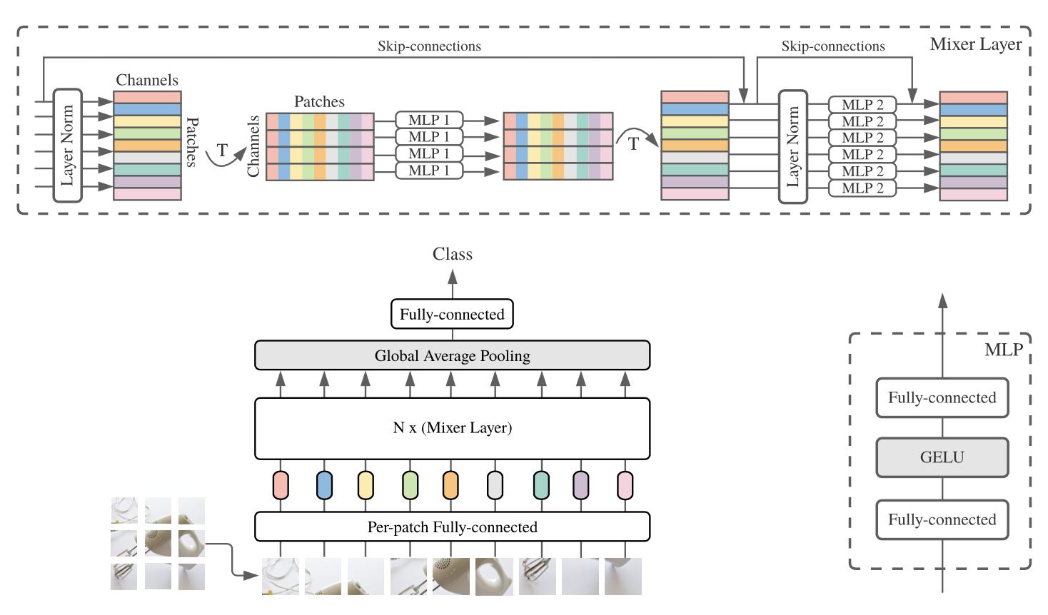
MLP-Mixer
Vision Transformer와 견줄만한 MLP 스타일의 network (CNN하고 다름)
자세한 내용은
[논문리뷰] 'MLP-Mixer: An all-MLP Architecture for Vision' 리뷰 + 구현(PyTorch)안녕하세요. 밍기뉴와제제입니다. 이번에 리뷰할 논문은 MLP-Mixer: An all-MLP Architecture for Vision 입니다. MLP만 가지고 image classification을 수행한다는 것 때문에 화제가 되었던 논문이기도 합니다. 물론 Batch Normalization같은 것들도 들어있습니다. MLP Mixer는 구조도 꽤 간단하고 필요한 parameter의 수가 적기 때문에 진입장벽(?)이 낮습니다. 그래서 PyTorch로 구현을 한 뒤 CIFAR-10 데이터셋 으로 학습시켜봤습니다.https://velog.io/@minkyu4506/%EB%85%BC%EB%AC%B8%EB%A6%AC%EB%B7%B0-MLP-Mixer-An-all-MLP-Architecture-for-Vision-%EB%A6%AC%EB%B7%B0-%EA%B5%AC%ED%98%84
코드
# -*- coding: utf-8 -*- import torch import torch.nn as nn #1단계 patch-wise 나눠주기 class Per_patch_Fully_connected(nn.Module) : def __init__(self, input_size, patch_size, C) : super(Per_patch_Fully_connected, self).__init__() self.S = int((input_size[-2] * input_size[-1]) / (patch_size ** 2)) #S는 패치 갯수 (몇개로 쪼개야되느냐) self.x_dim_1_val = input_size[-3] * patch_size * patch_size self.projection_layer = nn.Linear(input_size[-3] * patch_size * patch_size, C) #C사이즈로 토큰화 하기 #각 토큰은 각 지역에서 얻은 정보를 가지고 연산하는 것 def forward(self, x) : x = torch.reshape(x, (-1, self.S, self.x_dim_1_val)) return self.projection_layer(x) #2단계 Tocken-mixing MLP Block에서 연산 순서 #1. Layer normalization: token 별로 normalization #2. Transpose: SxC -> CxS #3. MLP #4. inverse-transpose: CxS -> SxC #5. Skip connection class token_mixing_MLP(nn.Module): def __init__(self, input_size): super(token_mixing_MLP, self).__init__() self.Layer_Norm = nn.LayerNorm(input_size[-2]) # C개의 값(columns)에 대해 각각 normalize 수행하므로 normalize되는 벡터의 크기는 S다. self.MLP = nn.Sequential( nn.Linear(input_size[-2], input_size[-2]), nn.GELU(), nn.Linear(input_size[-2], input_size[-2]) ) def forward(self, x): # layer_norm + transpose # [S x C]에서 column들을 가지고 연산하니까 Pytorch의 Layer norm을 적용하려면 transpose 하고 적용해야함. output = self.Layer_Norm(x.transpose(2, 1)) # transpose 후 Layer norm -> [C x S] 크기의 벡터가 나옴 output = self.MLP(output) # [Batch x S x C] 형태로 transpose + skip connection output = output.transpose(2, 1) return output + x class channel_mixing_MLP(nn.Module): def __init__(self, input_size): # super(channel_mixing_MLP, self).__init__() self.Layer_Norm = nn.LayerNorm(input_size[-1]) # S개의 벡터를 가지고 각각 normalize하니까 normalize되는 벡터의 크기는 C다 self.MLP = nn.Sequential( nn.Linear(input_size[-1], input_size[-1]), nn.GELU(), nn.Linear(input_size[-1], input_size[-1]) ) def forward(self, x): output = self.Layer_Norm(x) output = self.MLP(output) return output + x # input_size : [Batch, S, C] 크기의 벡터 class Mixer_Layer(nn.Module) : def __init__(self, input_size) : # super(Mixer_Layer, self).__init__() self.mixer_layer = nn.Sequential( token_mixing_MLP(input_size), channel_mixing_MLP(input_size) ) def forward(self, x) : return self.mixer_layer(x) # MLP-Mixer # Per_patch_Fully_connected, token_mixing_MLP, channel_mixing_MLP로 구성됨 # input_size : 입력할 이미지 사이즈. (Batch, C, H, W) 양식이다. 예를 들면 (1, 3, 224, 224). (3, 224, 224) 크기의 데이터로 넣어도 된다 # patch_size : 모델이 사용할 patch의 사이즈. 예를 들어 16 # C : desired hidden dimension. 예를 들어 16 # N : Mixer Layer의 개수 # classes_num : 분류해야하는 클래스의 개수 class MLP_Mixer(nn.Module): def __init__(self, input_size, patch_size, C, N, classes_num): super(MLP_Mixer, self).__init__() S = int((input_size[-2] * input_size[-1]) / (patch_size ** 2)) # embedding으로 얻은 token의 개수 self.mlp_mixer = nn.Sequential( Per_patch_Fully_connected(input_size, patch_size, C) ) for i in range(N): # Mixer Layer를 N번 쌓아준다 self.mlp_mixer.add_module("Mixer_Layer_" + str(i), Mixer_Layer((S, C))) # Glboal Average Pooling # Appendix E에 pseudo code가 있길래 그거 보고 제작 # LayerNorm 하고 token별로 평균을 구한다 self.global_average_Pooling_1 = nn.LayerNorm([S, C]) self.head = nn.Sequential( nn.Linear(S, classes_num), nn.Softmax(dim=1) ) def forward(self, x): if len(x.size()) == 3: x = torch.unsqueeze(x, 0) # 4차원으로 늘려줌. output = self.mlp_mixer(x) output = self.global_average_Pooling_1(output) output = torch.mean(output, 2) return self.head(output) if __name__ == '__main__': image_size = [50, 3, 256, 256] patch_size = 16 C = 512 N = 5 classes_num = 1000 model = MLP_Mixer(image_size, patch_size, C, N, classes_num) img = torch.randn(1, 3, 256, 256) pred = model(img) # (1, 1000)
Uploaded by
N2T


댓글 영역